Multiple plots#
Figanos also creates xr.plot.facetgrid.FacetGrid due to being wrapped around xarray plotting functions. This allows for multiple plots to be created at once. The following example shows how to create multiple timeseries and maps plots.
[1]:
# import necessary libraries
import cartopy.crs as ccrs
import numpy as np
import xarray as xr

import figanos.matplotlib as fg


# use ouranos style
fg.utils.set_mpl_style("ouranos")
Timeseries#
[2]:
# Create a xarray object from a NetCDF
url = "https://pavics.ouranos.ca//twitcher/ows/proxy/thredds/dodsC/birdhouse/disk2/cccs_portal/indices/Final/BCCAQv2_CMIP6/tx_max/YS/ssp585/ensemble_percentiles/tx_max_ann_BCCAQ2v2+ANUSPLIN300_historical+ssp585_1950-2100_30ymean_percentiles.nc"
opened = xr.open_dataset(url, decode_timedelta=False, engine="netcdf4")
[3]:
ds_time = opened.isel(lon=[500], lat=[150, 250])
im = fg.timeseries(
    {"p50": ds_time.tx_max_p50, "p90": ds_time.tx_max_p90},
    plot_kw={"p50": {"col": "lat"}, "p90": {"col": "lat"}},
    fig_kw={"figsize": (10, 4)},
    legend="edge",
    show_lat_lon=True,
)

[4]:
# Create fake scenarios
ds_time = ds_time[["tx_max_p10", "tx_max_p50", "tx_max_p90"]]
data = {
    "tasmax_ssp434": ds_time,
    "tasmax_ssp245": ds_time.copy() - 10,
    "tasmax_ssp585": ds_time.copy() + 10,
}

fg.timeseries(
    data=data,
    legend="facetgrid",
    show_lat_lon=False,
    fig_kw={"figsize": (9, 4)},
    plot_kw={
        "tasmax_ssp434": {"col": "lat"},
        "tasmax_ssp245": {"col": "lat"},
        "tasmax_ssp585": {"col": "lat"},
    },
    enumerate_subplots=True,
)
[4]:
<xarray.plot.facetgrid.FacetGrid at 0x7c5761f00b90>

Maps#
Create multiple maps plot with figanos wrapped around xr.plot.facetgrid.FacetGrid by passing the keys row and col in the argument plot_kw.
[5]:
# Select a time and slicing our starting Dataset
ds_space = opened[["tx_max_p50"]].isel(time=[0, 1, 2]).sel(lat=slice(40, 65), lon=slice(-90, -55))

# Defining a spatial projection
projection = ccrs.LambertConformal()

im = fg.gridmap(
    ds_space,
    projection=projection,
    plot_kw={"col": "time"},
    features=["coastline", "ocean"],
    frame=False,
    use_attrs={"suptitle": "description"},
    enumerate_subplots=True,
)

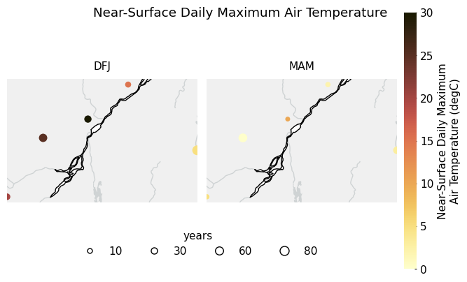
[7]:
names = ["station_" + str(i) for i in np.arange(5)]
lat = 45 + np.random.rand(5) * 3
lon = np.linspace(-76, -70, 5)
tas = np.array([[20, 25, 30, 15, 5], [5, 0, 10, 2, 3]])
yrs = np.array([[35, 65, 45, 25, 95], [15, 75, 10, 15, 50]])

attrs = {
    "units": "degC",
    "standard_name": "air_temperature",
    "long_name": "Near-Surface Daily Maximum Air Temperature",
}

tas = xr.DataArray(
    data=tas,
    coords={
        "season": ["DFJ", "MAM"],
        "station": names,
        "lat": ("station", lat),
        "lon": ("station", lon),
        "years": (("season", "station"), yrs),
    },
    dims=["season", "station"],
    attrs=attrs,
)
obs = xr.Dataset({"tas": tas})

# plot
fg.scattermap(
    obs,
    transform=ccrs.PlateCarree(),
    sizes="years",
    size_range=(25, 100),
    plot_kw={
        "col": "season",
    },
    features={
        "land": {"color": "#f0f0f0"},
        "rivers": {"edgecolor": "#cfd3d4"},
        "lakes": {"facecolor": "#cfd3d4"},
        "coastline": {"edgecolor": "black"},
    },
    fig_kw={"figsize": (7, 4)},
    legend_kw={"ncol": 4, "bbox_to_anchor": (0.15, 0.05)},
)
[7]:
<xarray.plot.facetgrid.FacetGrid at 0x7c579cc23a80>
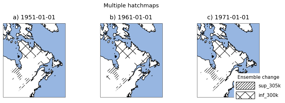
[8]:
sup_305k = ds_space.where(ds_space.tx_max_p50 > 305)
inf_300k = ds_space.where(ds_space.tx_max_p50 < 300)

im = fg.hatchmap(
    {"sup_305k": sup_305k, "inf_300k": inf_300k},
    plot_kw={
        "sup_305k": {
            "hatches": "////",  # hatches must be passed as a list of strings to matplotlib.pyplot.contourf
            "col": "time",
            "x": "lon",
            "y": "lat",
        },
        "inf_300k": {"hatches": "x", "col": "time", "x": "lon", "y": "lat"},
    },
    features=["coastline", "ocean"],
    frame=True,
    legend_kw={"title": "Ensemble change"},
    enumerate_subplots=True,
)

im.fig.suptitle("Multiple hatchmaps", y=1.08)
/tmp/ipykernel_2256/713627368.py:4: UserWarning: Only first variable of Dataset is plotted.
  im = fg.hatchmap(
/tmp/ipykernel_2256/713627368.py:4: UserWarning: Hatches argument must be of type 'list'. Wrapping string argument as list.
  im = fg.hatchmap(
/tmp/ipykernel_2256/713627368.py:4: UserWarning: Hatches argument must be of type 'list'. Wrapping string argument as list.
  im = fg.hatchmap(
/home/docs/checkouts/readthedocs.org/user_builds/figanos/conda/latest/lib/python3.14/site-packages/figanos/matplotlib/utils.py:332: UserWarning: Attribute "long_name" not found.
  suptitle = get_attributes(attr_dict["suptitle"], xr_obj)
[8]:
Text(0.5, 1.08, 'Multiple hatchmaps')
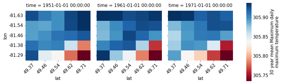
Heatmaps#
The keys row and col in the argument plot_kw can also be used to create a grid of heatmaps. This is done by wrapping Seaborn’s heatmap and FacetGrid
[9]:
ds_space = opened[["tx_max_p50"]].isel(time=[0, 1, 2]).sel(lat=slice(40, 65), lon=slice(-90, -55))

# Select a spatial subdomain
sl = slice(100, 100 + 5)
da = ds_space.isel(lat=sl, lon=sl).drop("horizon").tx_max_p50
da["lon"] = np.round(da.lon, 2)
da["lat"] = np.round(da.lat, 2)
fg.heatmap(da, plot_kw={"col": "time"})
/tmp/ipykernel_2256/501961280.py:5: FutureWarning: dropping variables using `drop` is deprecated; use drop_vars.
  da = ds_space.isel(lat=sl, lon=sl).drop("horizon").tx_max_p50
/home/docs/checkouts/readthedocs.org/user_builds/figanos/conda/latest/lib/python3.14/site-packages/seaborn/axisgrid.py:123: UserWarning: This figure includes Axes that are not compatible with tight_layout, so results might be incorrect.
  self._figure.tight_layout(*args, **kwargs)
[9]:
<seaborn.axisgrid.FacetGrid at 0x7c575bc45940>
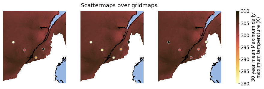
Plot over each other#
To overlay two facetgrid plots, you can create the first facetgrid with col or row and then loop through the ax of the first facetgrid and the xr.object to plot the second facetgrid.
[10]:
names = ["station_" + str(i) for i in np.arange(5)]
lat = 45 + np.random.rand(5) * 3
lon = np.linspace(-76, -70, 5)
tas = np.array(
    [
        [290, 300, 295, 305, 301],
        [275, 285, 277, 301, 345],
        [302, 293, 295, 292, 280],
    ]
)

attrs = {
    "units": "degK",
    "standard_name": "air_temperature",
    "long_name": ds_space.tx_max_p50.attrs["description"],
}

tas = xr.DataArray(
    data=tas,
    coords={
        "time": ds_space.time.values,
        "station": names,
        "lat": ("station", lat),
        "lon": ("station", lon),
    },
    dims=["time", "station"],
    attrs=attrs,
)
obs2 = xr.Dataset({"tas": tas})
[11]:
V_MIN = 280
V_MAX = 310
ds_space = opened[["tx_max_p50"]].isel(time=[0, 1, 2]).sel(lat=slice(40, 65), lon=slice(-90, -55))

im = fg.gridmap(
    ds_space,
    projection=projection,
    plot_kw={
        "col": "time",
        "xlim": (-77, -69),
        "ylim": (43, 50),
        "vmin": V_MIN,
        "vmax": V_MAX,
    },
    features=["coastline", "ocean"],
    frame=False,
)
for i, fax in enumerate(im.axs.flat):
    fg.scattermap(
        obs2.isel(time=i),
        ax=fax,
        transform=ccrs.PlateCarree(),
        plot_kw={
            "x": "lon",
            "y": "lat",
            "vmin": V_MIN,
            "vmax": V_MAX,
            "edgecolor": "grey",
            "add_colorbar": False,
        },
        show_time=False,
    )
im.fig.suptitle("Scattermaps over gridmaps", x=0.45, y=0.95)
/home/docs/checkouts/readthedocs.org/user_builds/figanos/conda/latest/lib/python3.14/site-packages/figanos/matplotlib/utils.py:288: UserWarning: Attribute "description" not found.
  title = get_attributes(attr_dict["title"], xr_obj)
/home/docs/checkouts/readthedocs.org/user_builds/figanos/conda/latest/lib/python3.14/site-packages/figanos/matplotlib/utils.py:288: UserWarning: Attribute "description" not found.
  title = get_attributes(attr_dict["title"], xr_obj)
/home/docs/checkouts/readthedocs.org/user_builds/figanos/conda/latest/lib/python3.14/site-packages/figanos/matplotlib/utils.py:288: UserWarning: Attribute "description" not found.
  title = get_attributes(attr_dict["title"], xr_obj)
[11]:
Text(0.45, 0.95, 'Scattermaps over gridmaps')
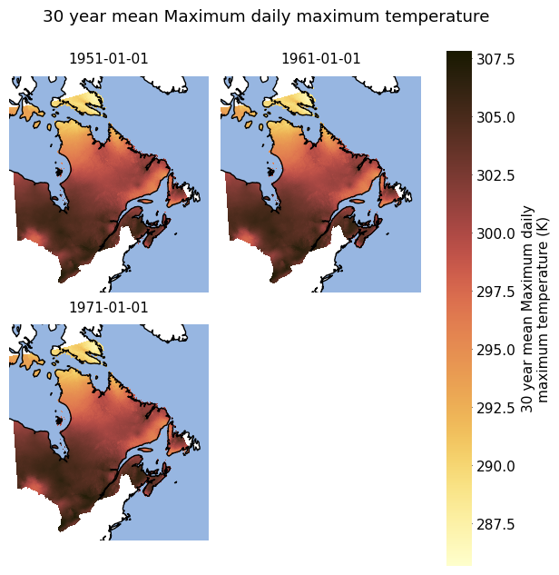
Limitations#
When the argument col_wrap is used for a facetgrid whose number of plots is not a multiple of col_wrap, no plot will be shown (see issue). set_extend needs to be passed to every axis in the facetgrid to avoid this issue.
[12]:
# Select a time and slicing for our starting Dataset
ds_space = opened[["tx_max_p50"]].isel(time=[0, 1, 2]).sel(lat=slice(40, 65), lon=slice(-90, -55))

im = fg.gridmap(
    ds_space,
    projection=ccrs.LambertConformal(),
    plot_kw={"col": "time", "col_wrap": 2},
    features=["coastline", "ocean"],
    frame=False,
    use_attrs={"suptitle": "long_name"},
    fig_kw={"figsize": (6, 6)},
)
for fax in im.axs.flat:
    fax.set_extent(
        [
            ds_space.lon.min().item(),
            ds_space.lon.max().item(),
            ds_space.lat.min().item(),
            ds_space.lat.max().item(),
        ]
    )
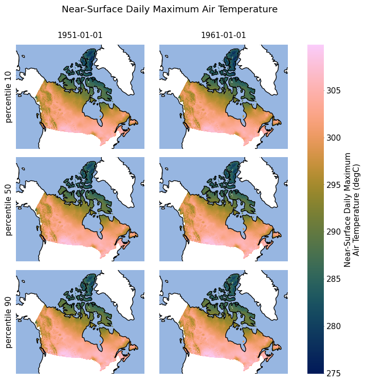
Xarray plots by default facetgrid ylabels to the right (next to the colorbar). The example below shows how to move the xlabels to the left.
[13]:
import numpy as np


op = opened.isel(time=[0, 1])
data = xr.DataArray(
    data=np.array([op.tx_max_p10.values, op.tx_max_p50.values, op.tx_max_p90.values]),
    dims=["percentile", "time", "lat", "lon"],
    coords={
        "percentile": [10, 50, 90],
        "time": op.time.values,
        "lat": op.lat.values,
        "lon": op.lon.values,
    },
    attrs={
        "units": "degC",
        "standard_name": "air_temperature",
        "long_name": "Near-Surface Daily Maximum Air Temperature",
    },
)

im = fg.gridmap(
    data,
    projection=ccrs.LambertConformal(),
    plot_kw={
        "col": "time",
        "row": "percentile",
    },
    features=["coastline", "ocean"],
    frame=False,
    use_attrs={"suptitle": "long_name"},
    fig_kw={"figsize": (8, 7)},
)

# Modify x-label positions (hardcoded in xarray.plot)
for fax in im.axs.flat:
    for txt in fax.texts:
        if len(txt.get_text()) > 0:
            txt.set_x(-1.2)
            txt.set_text("percentile " + txt.get_text())
            txt.set_rotation("vertical")
/home/docs/checkouts/readthedocs.org/user_builds/figanos/conda/latest/lib/python3.14/site-packages/figanos/matplotlib/plot.py:692: UserWarning: Colormap warning: Variable group not found. Use the cmap argument.
  get_var_group(da=plot_data),
/home/docs/checkouts/readthedocs.org/user_builds/figanos/conda/latest/lib/python3.14/site-packages/cartopy/io/__init__.py:242: DownloadWarning: Downloading: https://naturalearth.s3.amazonaws.com/110m_physical/ne_110m_ocean.zip
  warnings.warn(f'Downloading: {url}', DownloadWarning)
/home/docs/checkouts/readthedocs.org/user_builds/figanos/conda/latest/lib/python3.14/site-packages/cartopy/io/__init__.py:242: DownloadWarning: Downloading: https://naturalearth.s3.amazonaws.com/110m_physical/ne_110m_coastline.zip
  warnings.warn(f'Downloading: {url}', DownloadWarning)